Excel Basics: Conditional Formatting
Looking to change the color of a cell based on what’s in it? Read this tutorial and follow along in an example file as part of our Microsoft Excel Basics program. Let’s learn together!
-
Products and services that appear on CouchTripping.com may be from companies from which we receive compensation. Affiliated links allow us to earn revenue as an Amazon Associate. All available product choices may not be included, and we carefully consider the terms/rules of how products may be displayed or advertised at all times.
Products are reviewed fairly and objectively based on customer satisfaction, price, competition, features, and a number of other factors as well. Any ratings that may appear are based on the opinion of CouchTripping.com and its staff in good faith to provide the best product options for the described needs/scenario.
In Excel Basics, we aim to cover some tips to help get you started in your pursuit of adding more complex functionality into your spreadsheets, whether they be for budgeting, data entry, project tracking, or anything else.
Today, we’ll be helping you learn about conditional formatting, which can change the color or font of a cell based on what’s in it or around it.
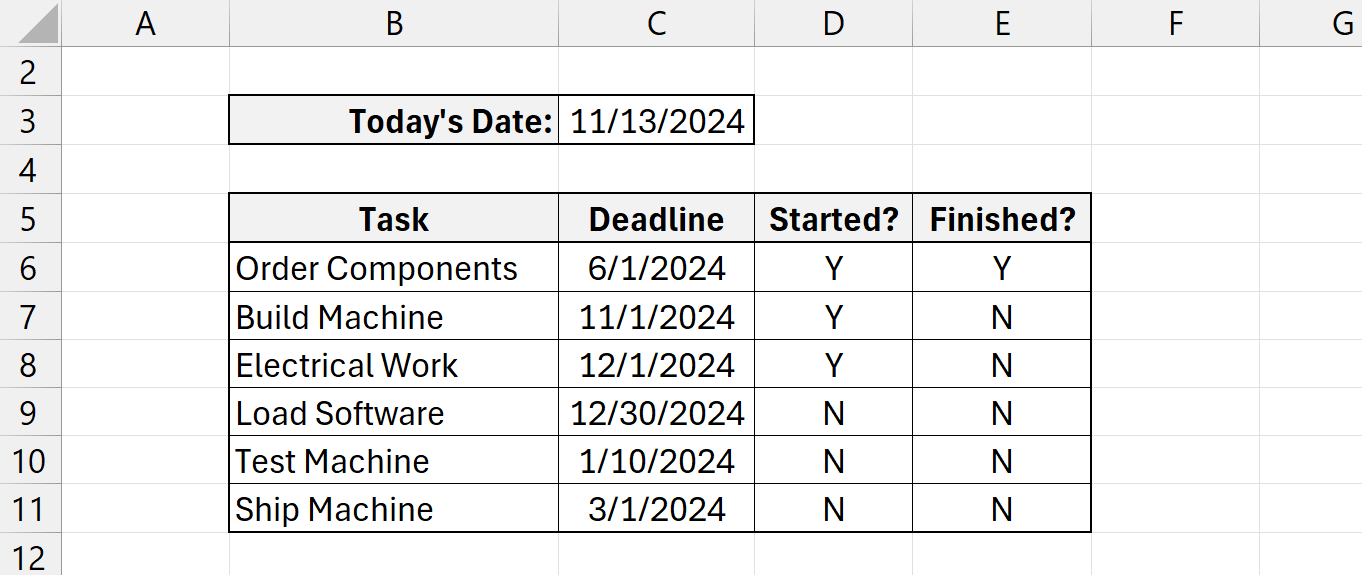
The example we will be covering today will be a mock status sheet for tracking/managing a small machine-building project.
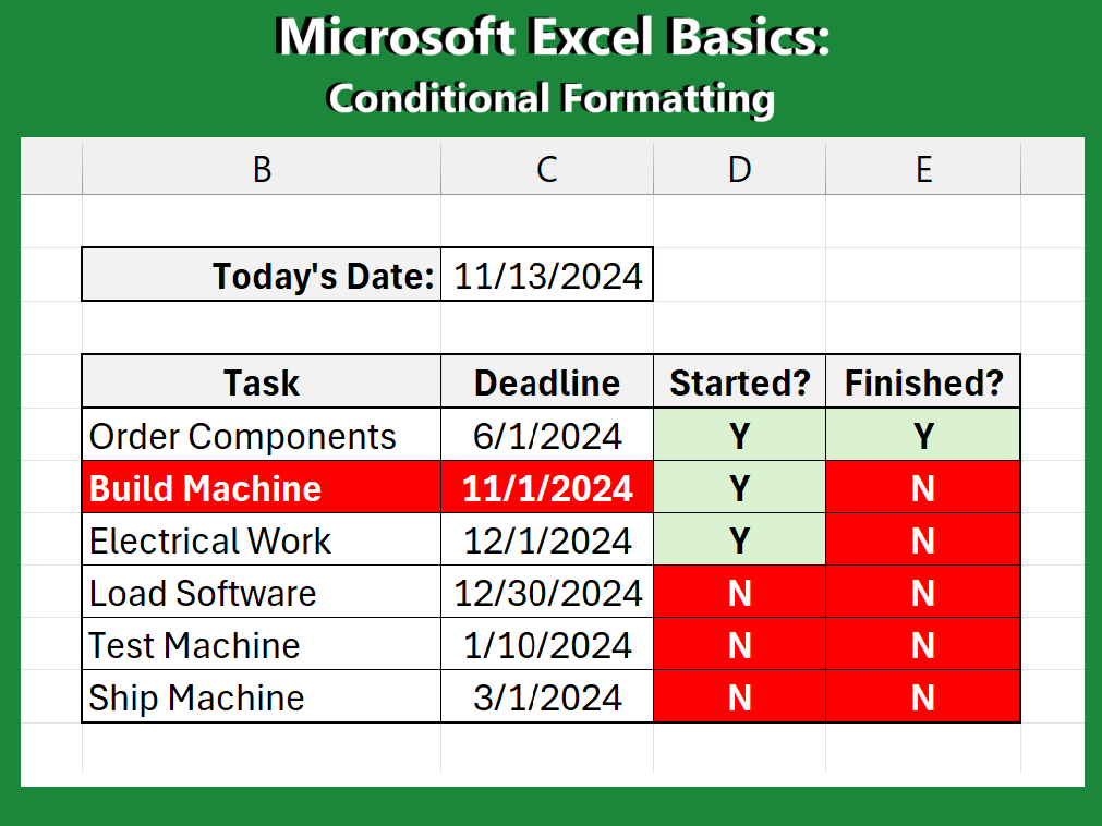
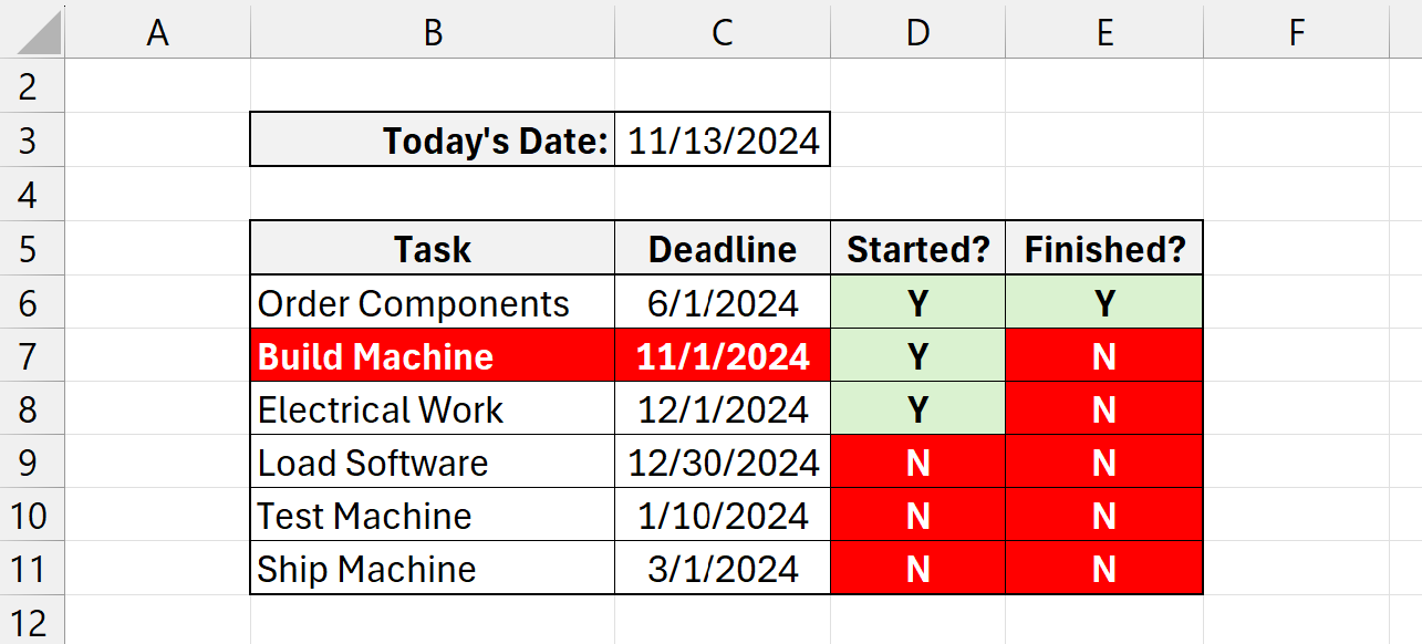
In this example, we have some tasks that must be done for the project laid out in a table, and each task has its own deadline and statuses for whether it has been started or finished. Our goal is to change the colors and fonts of the table’s cells based on each task’s statuses and deadline.
Above this table, we have the current date. This date will be static for the purposes of this example, but you can also set up your table to use today’s actual date with the TODAY() function instead. We will use this date to determine if we have already passed the deadline we set for a task.
If you want to follow along with this example in Excel, feel free to download the file using the following link:
Conditional Formatting - Test File
The test file contains the finished version of the example we will be covering, as well as an unfinished example if you want to practice while you read this guide. At the end, you can then compare your version to what was already in the file to see how you did.
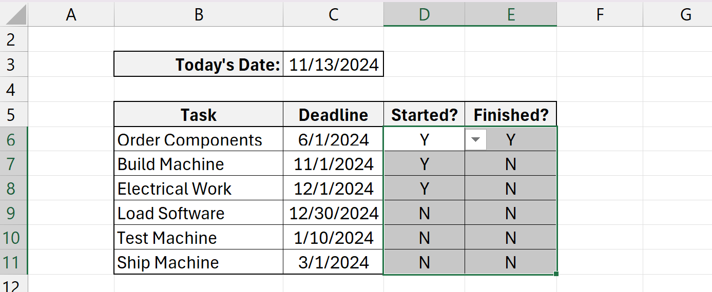
The “Started?” and “Finished?” columns in this table use values of “Y” and “N” to indicate “Yes” and “No,” respectively. The “Y” and “N” values are also selectable in these columns via dropdown lists, which you can learn more about how to set up in our article here.
Let’s start by using conditional formatting to change the color of these status columns.
First, select the cells in the “Started?” and “Finished?” columns.
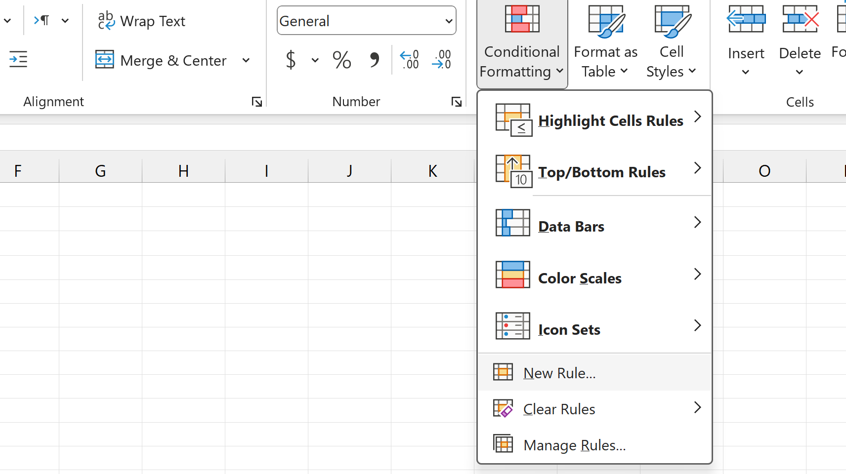
Then, navigate to Home —> Conditional Formatting at the top of the screen. Click on the option in Conditional Formatting called “New Rule.”
This will open up the New Formatting Rule window.
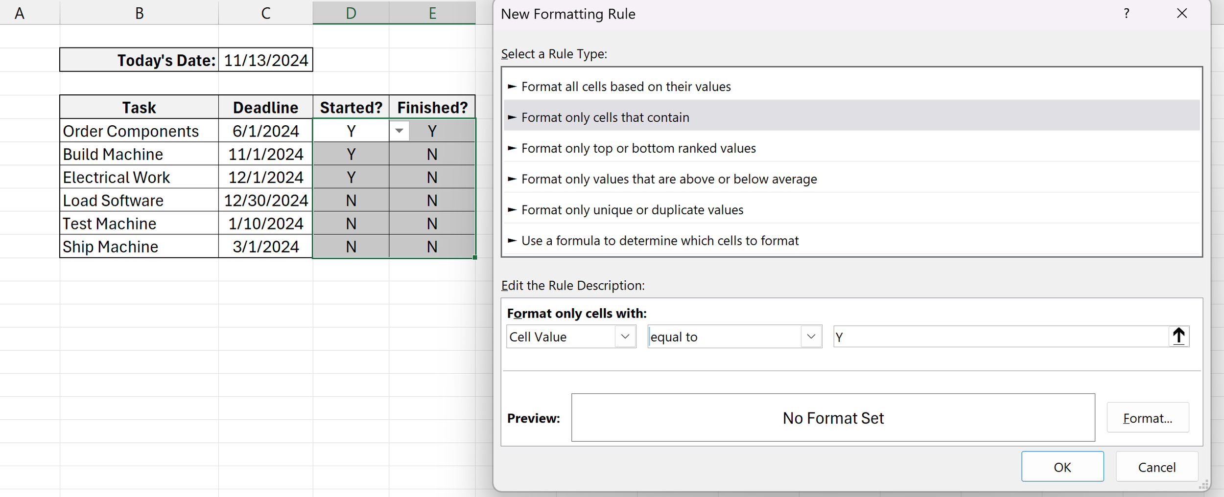
In the New Formatting Rule window, we are shown all the different options that we can use to change the color/font formatting of the selected cells. We can format cells based on what’s in them or we can use a formula to also format them based on what’s around them.
For these selected cells, we want to change the color of cells containing a “Y” to be green and the cells containing a “N” to be red. This will help us tell the difference between the two.
To do this, select the “Format only cells that contain” rule type from the list. For our rule description, let’s set it up such that cells are only formatted if their cell values are equal to Y and N, respectively.
Let’s start with “Y.”
Underneath the “Format only cells with” option, choose “equal to” from the dropdown list instead of the default “between” option. Then, enter a Y in the field to the right.
This sets up our rule, but now we need to tell Excel to format these cells differently if the criteria are met. To change the formatting, click on the “Format…” button in the bottom right corner.
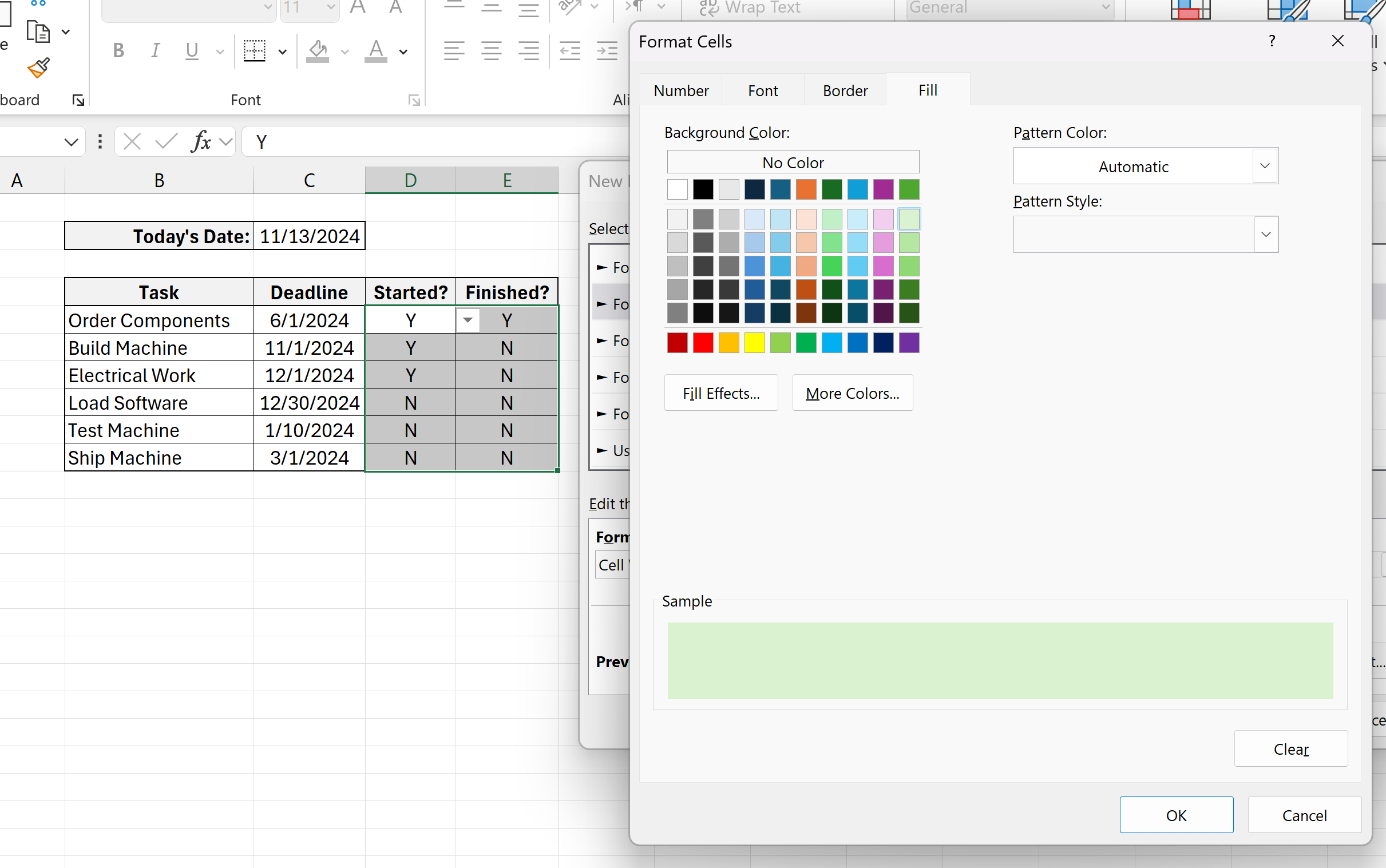
This will bring up the Format Cells window. In this window, you can choose to change a cell’s font, bordering, fill, and numbering.
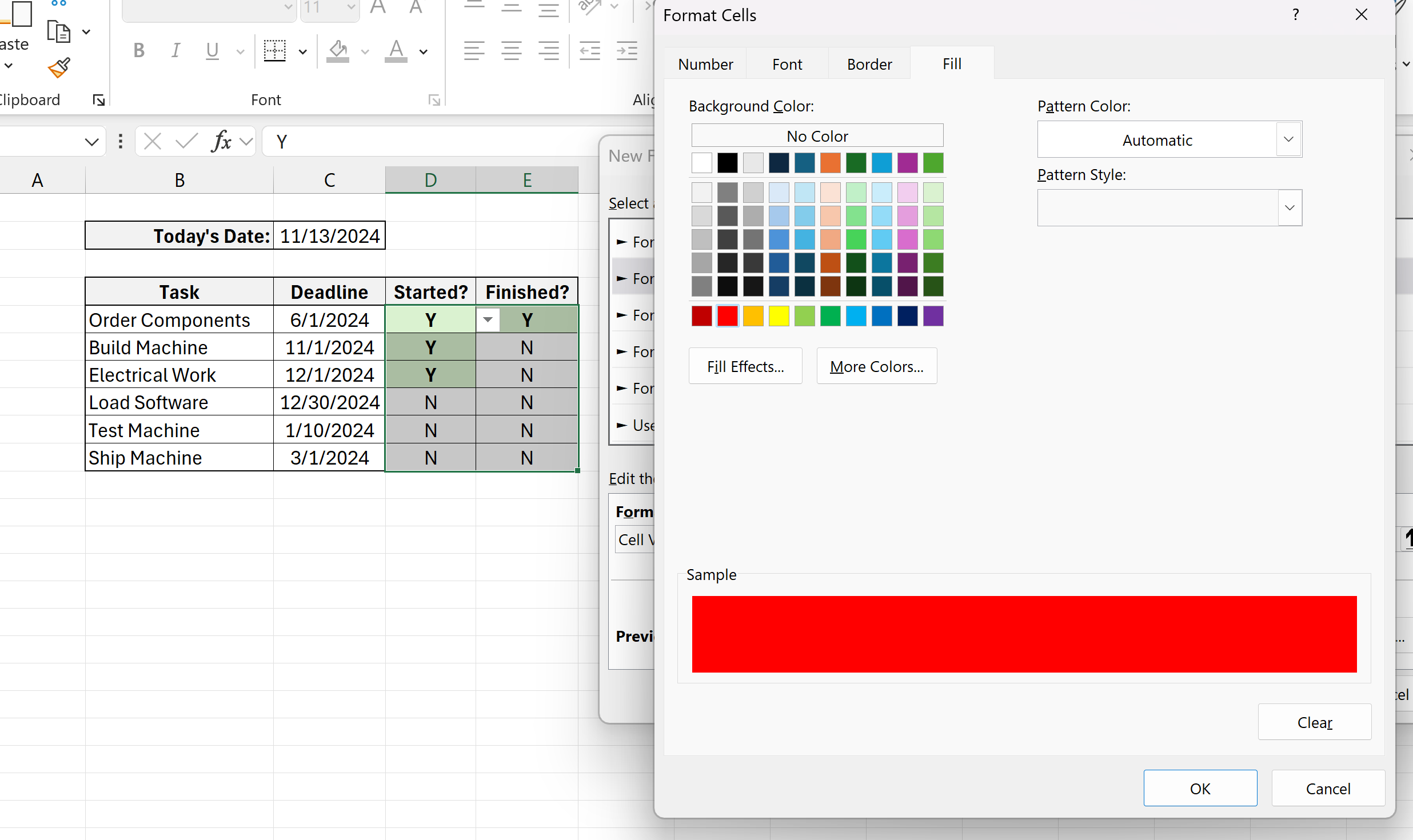
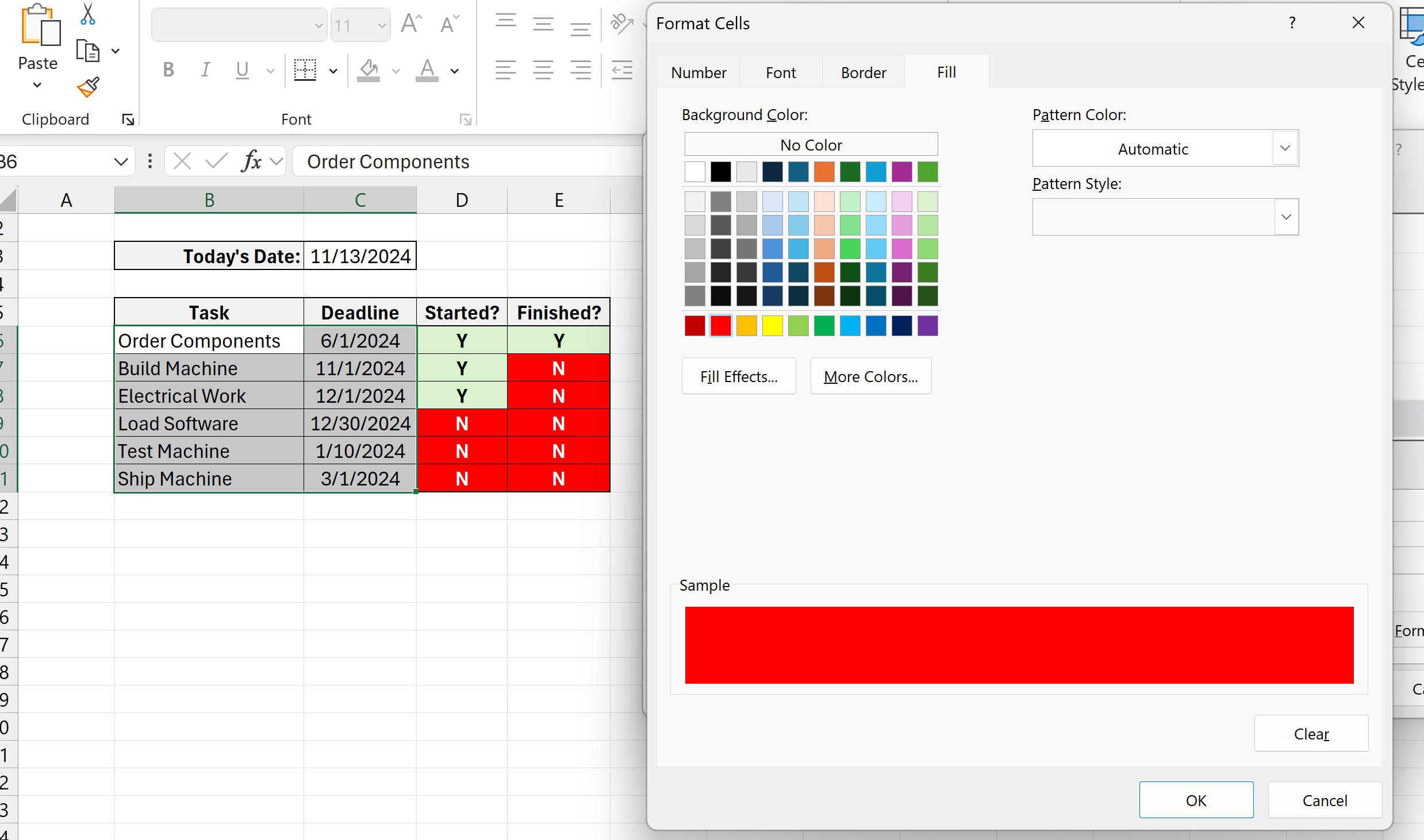
In the Fill category, let’s change the cell to be green, picking one of the available options from the pallet.
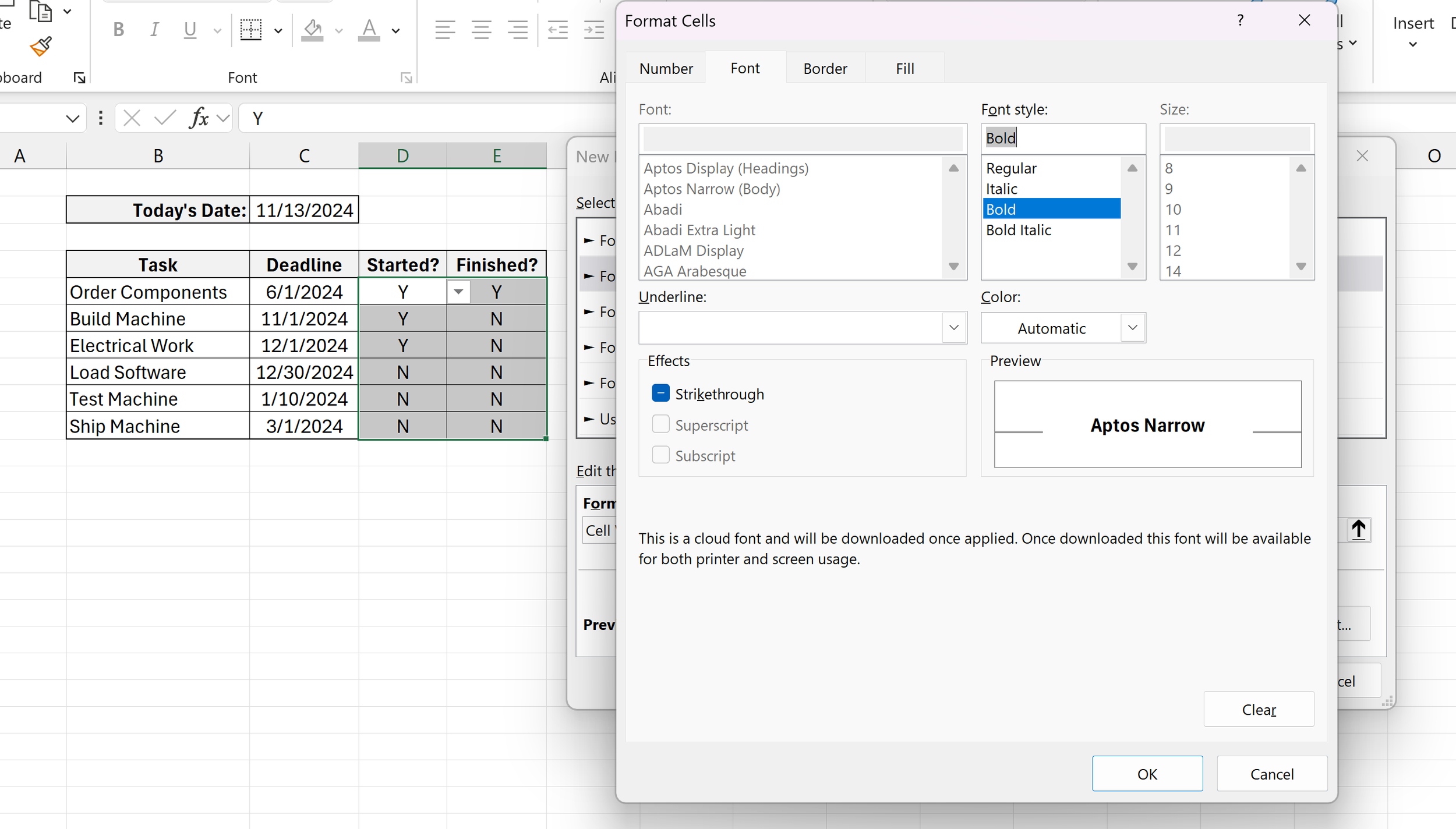
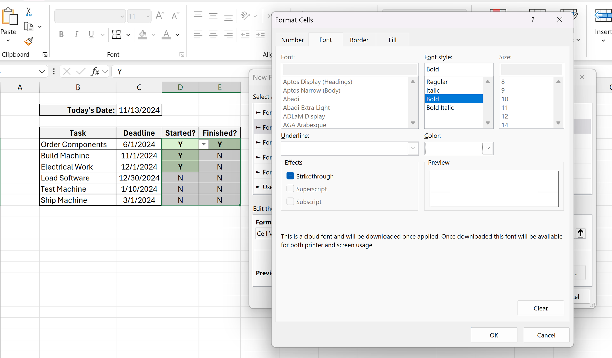
Looking at the preview sample at the bottom, this text may be a little bit harder to read than before, so let’s also navigate to the Font category and choose “Bold” for the Font Style.
Now, we’re good to go!
Click OK on all open windows to set your rule, and any cells in the status columns with a “Y” in them should now use our new formatting.
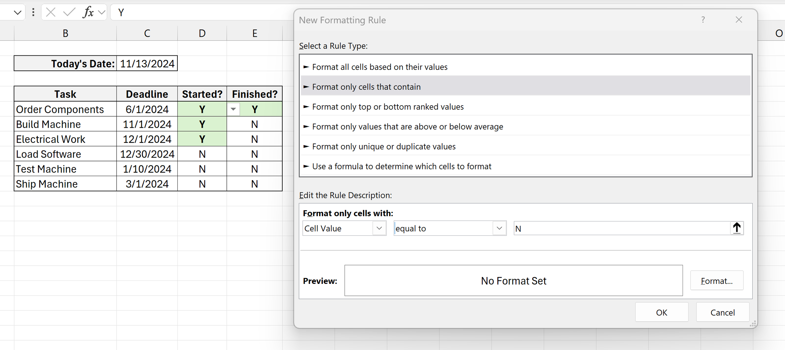
Let’s then keep the cells highlighted and repeat these steps to turn the cells with a “N” in them red.
Navigate to Conditional Formatting once more and click New Rule to open up the New Formatting Rule window. Select the same options as before, substituting in a “N” instead of a “Y.” in the field to the right.
Click the “Format…” button in the bottom right corner to open up the Format Cells window.
In our Fill category, let’s change the cells to be red this time.
Like last time, our text in the preview is now a little harder to read. Let’s fix this by navigating to the Font category. Choose “Bold” for the Font Style and change the Font Color from “Automatic” to a contrasting white color.
Click OK on all open windows to set this second rule, and any cells in the status columns with a “N” in them should now show as red.
Now, let’s try changing the formatting of a cell based on what’s in our other cells!
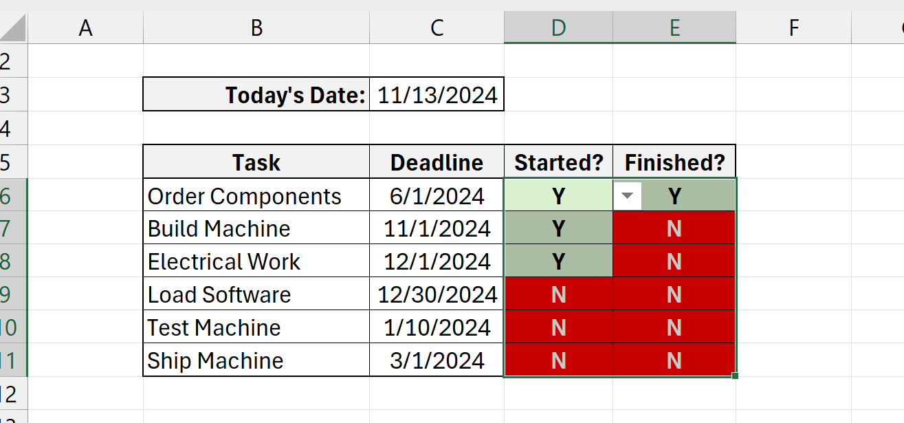
For instance, let’s say that we started one of our tasks in the list, but we haven’t finished it by the deadline we set. It might be helpful to highlight these cells red too so we can see where we’re falling behind.
Highlight the first two columns of the table and click Conditional Formatting —> New Rule to open the New Formatting Rule window as before.
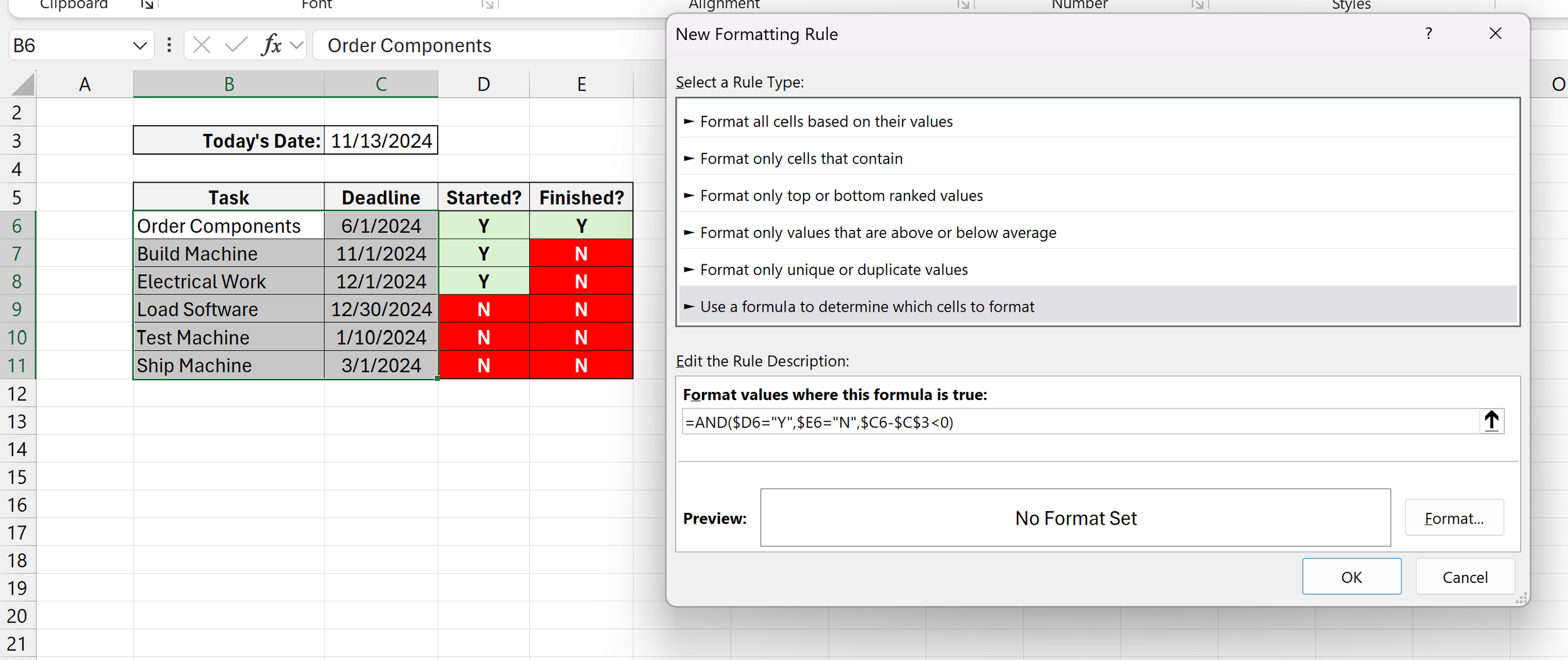
This time, because we’re going to be changing the formatting based on what’s in other cells, we’re going to pick a different Rule Type from the list: “Use a formula to determine which cells to format.”
Using a formula allows us to tell Excel exactly what we want our conditions to be to change the formatting of the cells.
For this example, we’re going to want to look at the values “Started?” and “Finished?” columns of our table to see if the task has been started but not finished. Then, if we find a scenario where this is the case, we also want to check if today’s date is greater than our deadline that we set. This lets us know that this task is late.
For those new to Excel formulas, coming up with the formula we need may be a little tricky at first, but let’s go through how to build it.
In Excel, the AND() function may be used to tell you if certain conditions are all being met at the same time.
If you tell the AND() function, “Check if the value of Cell One is ‘5’ and the value of Cell Two is ‘3,’” the function will only return a result of TRUE if these values are present. If Cell One instead had a “7” in it, the AND() function would see that not all of the conditions are being met, and it would return a result of FALSE, even if the value in Cell Two was correct.
As such, we can use the AND() function to check if the “Started?” column has a “Y” in it and if the “Finished?” column has a “N” in it, indicating that the task has been started but not finished.
The AND() function that checks this might look something like this:
AND(D6=”Y”, E6=”N”)
D6 represents the first value in our “Started?” column, and E6 represents the first value in our “Finished?” column. This formula will only return TRUE if a task has been started but not finished.
But, we also need to check if today’s date has already passed our set deadline.
Well, we can add more conditions to check for this inside of the AND() function. We can add as many conditions as we like, separating them with commas.
Let’s add this condition to our previous AND() function now to see how that would look:
AND(D6=”Y”, E6=”N”, C6 - $C$3 < 0)
The only thing we’ve added is at the end, where we are subtracting today’s date ($C$3) from the first deadline in our column (C6) and checking if this value is less than 0 or not.
You may have noticed the dollar signs ($’s) added for today’s date in the equation. This is because we want to make sure it is always using the correct cell.
A dollar sign in front of a column’s letter says, “Always use this column.” A dollar sign in front of a row’s number says, “Always use this row.”
When we apply our formula to all our highlighted cells, anything without a dollar sign will change from row-to-row, ensuring that each row’s deadline and status information stay together. But, we don’t want today’s date to change for each row too, so we have to tell Excel to keep this the same each time.
Now, let’s put this formula in for our New Formatting Rule:
Click the “Format…” button in the bottom right corner to open up the Format Cells window.
In our Fill category, let’s change the cells to be red once more.
Like before, choose “Bold” for the Font Style and change the Font Color from “Automatic” to a contrasting white color.
Click OK on all open windows to set this final rule, and any tasks that have been started, not finished, and are past their deadline should now show as red.
With all our conditional formatting rules all set up for these cells, feel free to change the values as you please to test out how all of the different rules interact.
If you ever want to change or remove one of the conditional formatting rules, navigate to the Conditional Formatting menu once more, and choose the option labeled, “Manage Rules.”
This will allow you to edit, remove, or add rules as you wish, configuring the colors and fonts of your cells to your heart’s content!
And that about wraps it up for this example! If you liked this guide or want to learn more about Microsoft Excel, feel free to read more of our content in the Excel Basics program, or explore some of our most recent articles on the site below.
