Excel Basics: Checkmarks for Task Completion
Looking to add a checkbox or change the color of a cell based on interactive checkmarks? Read this tutorial and follow along in an example file as part of our Microsoft Excel Basics program. Let’s learn together!
-
Products and services that appear on CouchTripping.com may be from companies from which we receive compensation. Affiliated links allow us to earn revenue as an Amazon Associate. All available product choices may not be included, and we carefully consider the terms/rules of how products may be displayed or advertised at all times.
Products are reviewed fairly and objectively based on customer satisfaction, price, competition, features, and a number of other factors as well. Any ratings that may appear are based on the opinion of CouchTripping.com and its staff in good faith to provide the best product options for the described needs/scenario.
In Excel Basics, we aim to cover some tips to help get you started in your pursuit of adding more complex functionality into your spreadsheets, whether they be for budgeting, data entry, project tracking, or anything else.
Today, we’ll be helping you learn about interactive checkmarks, which can change the color of cells based on whether the checkbox is checked or not.
The example we will be covering today will be a fairly simple list of spring-cleaning tasks for around the home.
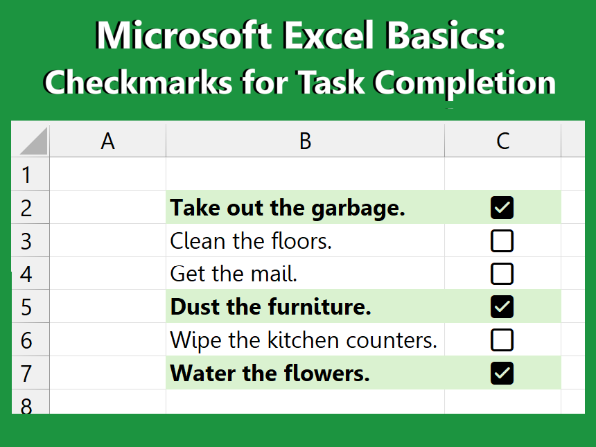
In this example, we have some tasks that we want to put checkboxes next to so that we can check to see if we have already done them or not. We also want these cells to become highlighted green to better let us know when they are done.
If you want to follow along with this example in Excel, feel free to download the file using the following link:
The test file contains the finished version of the example we will be covering, as well as an unfinished example if you want to practice while you read this guide. At the end, you can then compare your version to what was already in the file to see how you did.
1. Insert Checkboxes
First, let’s begin by adding in some checkboxes next to each task in the list.
To do so, we can use Excel’s built-in Checkbox tool inside of the Insert menu.
Clicking on the Checkbox option inserts a checkbox into the selected cell(s).
Go ahead and insert checkboxes into the column next to our starting task list.
When a checkbox has been checked, the value of the cell becomes “TRUE.”
When a checkbox is left unchecked, the value of the cell remains “FALSE.”
Knowing these values is important for any formulas you may want to create involving checkboxes.
2. Conditional Formatting
Next, we will use conditional formatting to make it so that any tasks that have been completed turn green to further indicate that they are done.
If you want to learn more about how to use conditional formatting, feel free to check out our previous article here.
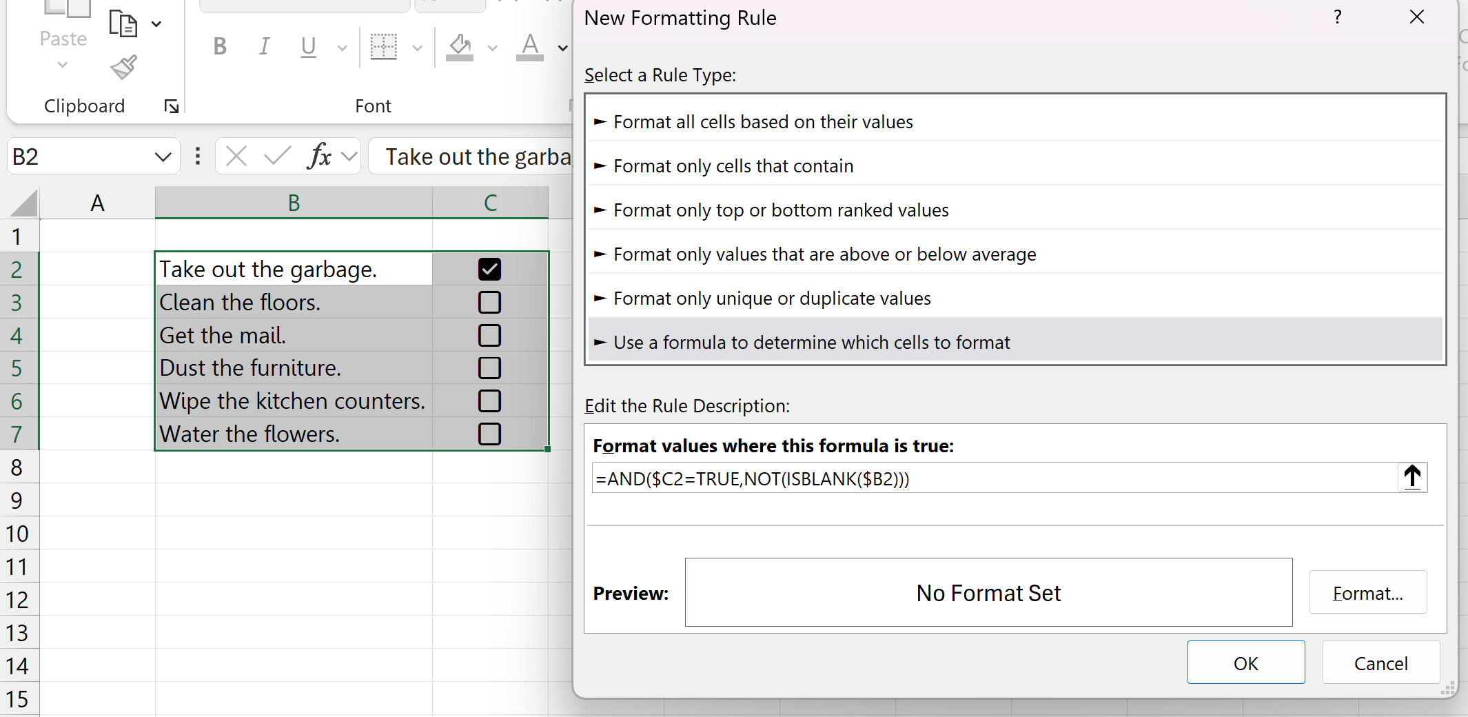
Highlight all of the cells in our list so far, navigate to Conditional Formatting, and select New Rule.
If we were just formatting the cells with the checkboxes to turn green, we could easily use our “Format only cells that contain” rule type to look for a TRUE or FALSE value in the cell.
But, in this example, we also want to turn the cells with the tasks in them green as well.
Instead, let’s select the “Use a formula” rule type.
3. Formula for Conditional Formatting
Now, let’s break down how to get the formula we will be using for this example.
We want to tell Excel to turn both columns green if the checkbox is checked for the task. From earlier, we know that when a checkbox is checked, the value of the cell ($C2) is TRUE. So, with this in mind, we know that one of our conditions should be:
$C2 = TRUE
Recall from our conditional formatting lesson that the dollar sign ($) in front of the “C” means that Excel should always be looking at the C column and nothing else.
We could get away with just checking for this condition only, but let’s make it a little more interesting.
In our formula, we can also make sure that a checkmark only turns the cells green if a task is actually present in the task column (not blank).
To do this, we want to use two different functions nested inside of each other: the NOT() function and the ISBLANK() function.
The NOT() function returns the opposite value of whatever condition is inside of it. For example, if we put something inside of the NOT() function that was a TRUE statement, the NOT() function would flip it and make it FALSE instead.
The ISBLANK() function checks to see if the cell you’re looking at is blank or not. If the cell is blank, it returns a TRUE statement. If the cell is not blank, it returns a FALSE statement.
But, we want to use the NOT() function to flip the value of the ISBLANK() function, because what we really want to know is if the cell is not blank.
So, let’s put it all together:
=AND($C2 = TRUE, NOT(ISBLANK($B2)))
Our first condition is the $C2 = TRUE condition from before. Our other condition, separated by the comma, must then also equal TRUE at the same time for our AND() function to work.
In the second condition, we’re asking Excel to tell us if our task ($B2) is blank, and Excel is telling us FALSE, it is not blank. The NOT() function then flips this FALSE to a TRUE so that our formula works properly, and both conditions are TRUE at the same time.
4. Choose Cell Color & Font
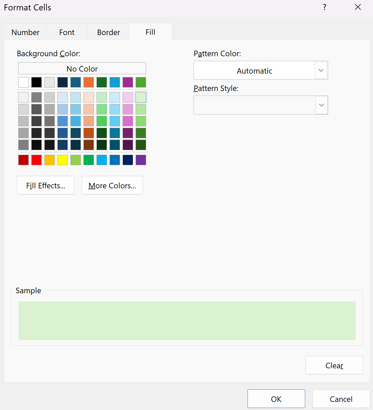
Click the “Format…” button to open up the Format Cells window.
On the Fill tab, select a green color to highlight the cells with.
Then, navigate to the Font tab.
Select Bold from the Font Style dropdown, and then click “OK” on all open windows to set the conditional formatting rule.
5. Apply the Formatting Rule
With the rule applied to all cells in our list, task cells and checkbox cells will now highlight as green when checkmarks are present. Pretty neat!
You can also try deleting a task from the list next to a checked checkbox to test out our second condition in the formula. If a task is not present, the cells should no longer be highlighted green.
And that about wraps it up for this example! If you liked this guide or want to learn more about Microsoft Excel, feel free to read more of our content in the Excel Basics program, or explore some of our most recent articles on the site below.


