Excel Basics: Dynamic Drop-Down Lists
Looking to add a dynamic drop-down menu into your Excel file that changes based on other inputs? Read this tutorial and follow along in an example file as part of our Microsoft Excel Basics program. Let’s learn together!
-
Products and services that appear on CouchTripping.com may be from companies from which we receive compensation. Affiliated links allow us to earn revenue as an Amazon Associate. All available product choices may not be included, and we carefully consider the terms/rules of how products may be displayed or advertised at all times.
Products are reviewed fairly and objectively based on customer satisfaction, price, competition, features, and a number of other factors as well. Any ratings that may appear are based on the opinion of CouchTripping.com and its staff in good faith to provide the best product options for the described needs/scenario.
In Excel Basics, we aim to cover some tips to help get you started in your pursuit of adding more complex functionality into your spreadsheets, whether they be for budgeting, data entry, project tracking, or anything else.
Today, we’ll be helping you add a dynamic dropdown menu into your Excel file, which can change the available options in the dropdown based on other inputs in your sheet.
If you want to learn more about creating a basic dropdown menu, you can also refer to our previous edition of Excel Basics at the following link here.
The example we will be covering today will be a basic schedule and task assignment list.
We have some names of people on the left, and we want to create some dynamic dropdowns that show us the tasks they’ll be able to perform if they’re only available on certain days. On the right, we have some tasks that can be done only on certain days of the week.
If you want to follow along with this example in Excel, feel free to download the file using the following link:
The test file contains the finished version of the example we will be covering, and you can start a new sheet within the file if you want to practice while you read this guide. At the end, you can then compare your version to what was already in the file to see how you did.
The table on the right can be organized any way that you choose, as long as you can determine which items go with each category.
Our goal is to make the fields in the “Day Available” column have a dropdown list for the days of the week (Monday, Tuesday, etc.). Then, we want to create a dynamic dropdown list in the “Task” column that looks at the day in the previous column to only show tasks that are available for that particular day.
To do this, we have to first give names to our data ranges in the table to the right. Essentially, we will be highlighting certain cells and telling Excel what we want to call them. Let’s start with the days of the week.
Highlight the first row of the table to the right with the different days of the week, and right-click to view the available options. The one we’re looking for is called “Define Name.”
Note: You can also use the “Name Manager” tool from the top of the screen (under “Formulas”) if you want to delete a name or just add them using a different method.
Click on the “Define Name” option after right-clicking to bring up the “New Name” window.
In the “New Name” window, we want to choose a name that accurately describes the data we selected, that way we know what we’re referring to when we use the name somewhere else. For the days of the week, let’s choose to use the name “WEEKDAYS.”
Now, any time we use the formula “=WEEKDAYS” in the sheet, Excel will know which cells we’re talking about without us having to highlight them again. Pretty neat!
We can then do the same thing for each task list associated with the days of the week. Highlight the tasks that can only be done on Monday, right-click, and then choose “Define Name.”
Type the name “Monday” into the “New Name” window. It should exactly match the way you typed it in the first row.
Now, any time we want to refer to these cells, we can just call them “Monday.”
Repeat these steps for each other day of the week, until you have names for “Tuesday” tasks, “Wednesday” tasks, etc.
With all of our cells in the table on the right in named groups, we can now start working on our main table on the left.
Recall from our previous tutorial on adding a dropdown list into your Excel sheet, we can use the “Data Validation” tool to tell Excel what values are allowed in certain cells.
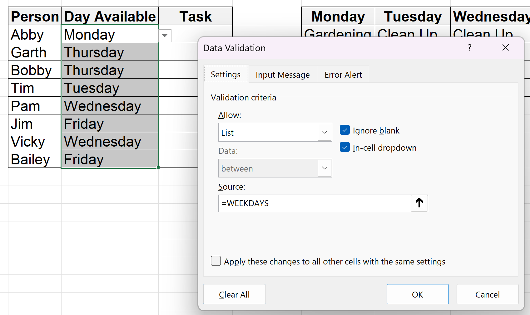
First, we will add a dropdown menu with the different days of the week into the “Day Available” column. Click on the “Data Validation” tool with this column highlighted to open the Data Validation window.
Set up the "Day Available” cells to allow only a “List.” The “Source” for this list will be the named group we made for the days of the week called “WEEKDAYS.” We don’t have to highlight these cells because we already told Excel which ones we’re talking about.
Then, we want to highlight the cells in the “Task” column and set up Data Validation for these cells as well.
These cells are set up a little differently. We still want these cells to pull from a list, but these dynamic dropdown lists will change from cell to cell, depending on what’s in the “Day Available” column.
To do this, we need to use the “=INDIRECT()” function built into Excel.
The INDIRECT() function tells Excel to look at a cell and see what’s in it. Then, it tries to see if this value can be used as a reference to something else it knows. (If it can’t find a reference, it shows an error.)
So, because we went through and named each task group by their day of the week (Monday, Tuesday, etc.), we can then use the INDIRECT() function to look at the day of the week in the “Day Available” column, find our named list in the table to the right, and give us a dynamic dropdown list of just those cells.
Go ahead and set up Data Validation for the first cell in the “Task” column to indirectly reference the cell next to it. Then, copy this Data Validation to the rest of the cells in the “Task” column.
The results should look similar to the ones below.
And voila! You now have a dynamic dropdown list that changes based on what’s in the cell next to it. Tasks will only show up for the days of the week they have been associated with.
We can then hide the columns of our table to the right so that we only see our main table with the dropdowns.
And that about wraps it up for this example! If you liked this guide or want to learn more about Microsoft Excel, feel free to read more of our content in the Excel Basics program, or explore some of our most recent articles on the site below.


